
What Is a Dynamic List in Excel?
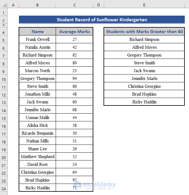
A dynamic list updates automatically when any value in the original data set is changed or new values are added. We have a list of the names of all the students who got marks greater than 60 in an exam.
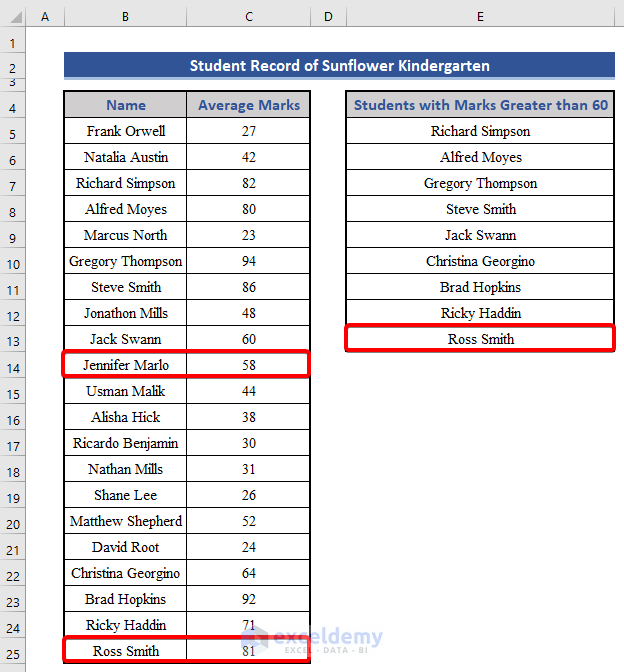
If you change the marks of Jennifer Marlo from 68 to 58 and add a new student called Ross Smith with a score of 81 in the table, the list will adjust itself automatically.
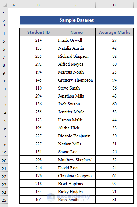
We’ll use a starting dataset with the Student IDs, Names, and Marks.
The FILTER function is available in Office 365 only.
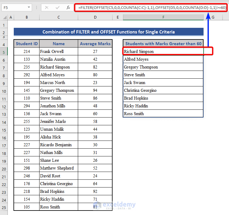
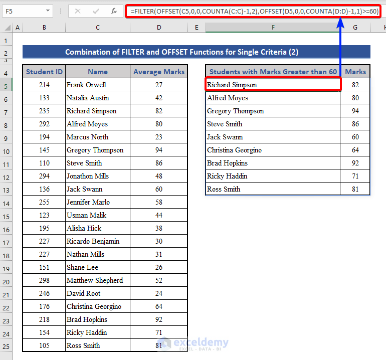
Case 1 – Based on Single CriteriaLet’s make a dynamic list of the students whose average marks are greater than or equal to 60.
Use the following formula:
=FILTER(OFFSET(C5,0,0,COUNTA(C:C)-1,1),OFFSET(D5,0,0,COUNTA(D:D)-1,1)>=60)
Explanation of the Formula:
Note:
If you want to get the marks along with the names in the list, change the fifth argument of the first OFFSET function from 1 to 2.
=FILTER(OFFSET(C5,0,0,COUNTA(C:C)-1,2),OFFSET(D5,0,0,COUNTA(D:D)-1,1)>=60)
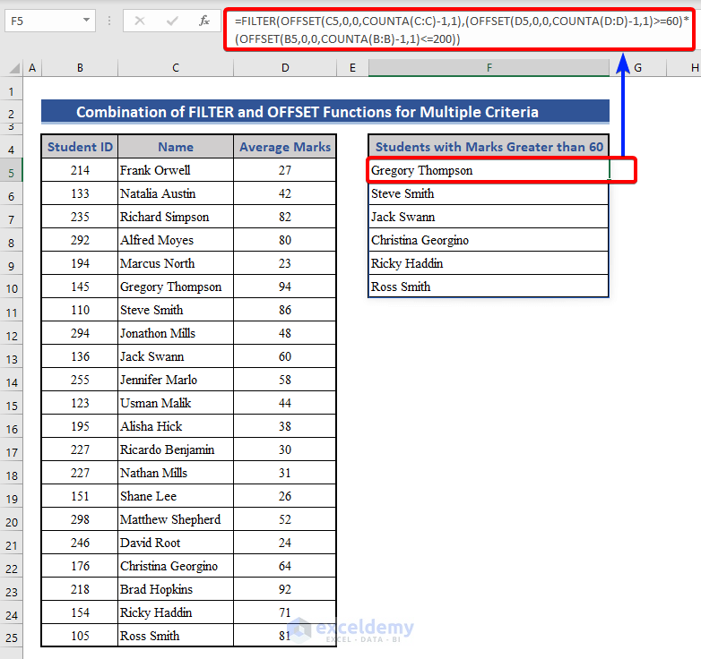
We’ll make a dynamic list of the students who got marks more than or equal to 60, but whose IDs are less than or equal to 200.
You can use this formula:
=FILTER(OFFSET(C5,0,0,COUNTA(C:C)-1,1),(OFFSET(D5,0,0,COUNTA(D:D)-1,1)>=60)*(OFFSET(B5,0,0,COUNTA(B:B)-1,1)<=200))
Explanation of the Formula:
Here we’ve multiplied two dynamic ranges of criteria, (OFFSET(D5,0,0,COUNTA(D:D)-1,1)>=60)*(OFFSET(B5,0,0,COUNTA(B:B)-1,1)<=200)
If you have more than 2 criteria, multiply all the ranges of criteria in the same way.
The rest is the same as the previous example (of single criteria). The OFFSET function in combination with the COUNTA function has been used to keep the formula dynamic.
Note:
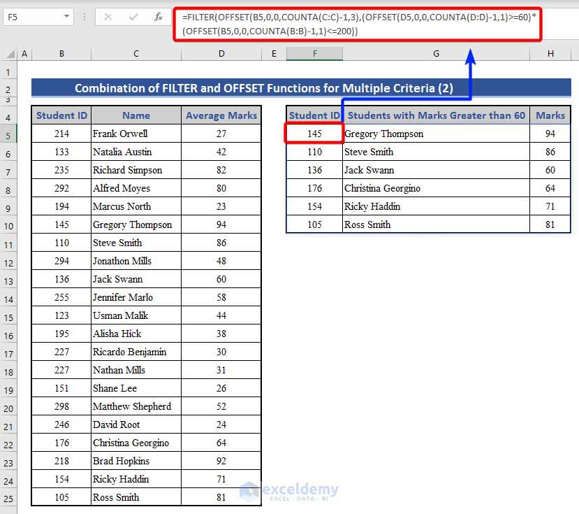
If you want to see all the columns in the list (Columns B, C, and D in this example), change the first argument of the first OFFSET function to the first column (B5 in this example), and the fifth argument to the total number of columns (3 in this example).
=FILTER(OFFSET(B5,0,0,COUNTA(C:C)-1,3),(OFFSET(D5,0,0,COUNTA(D:D)-1,1)>=60)*
(OFFSET(B5,0,0,COUNTA(B:B)-1,1)<=200))
Read More: How to Create Dynamic List From Table in Excel
Method 2 – Using INDEX-MATCH with Other Functions (For Old Versions)These formulas are array formulas. To apply them in older versions of Excel, you need to press Ctrl + Shift + Enter instead of just Enter.
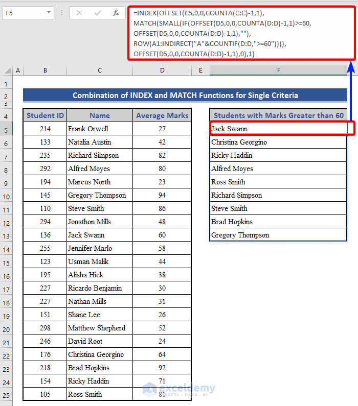
Case 1 – Based on Single CriteriaThe formula to create a dynamic list of the students who got more than or equal to 60 will be:
=INDEX(OFFSET(C5,0,0,COUNTA(C:C)-1,1),MATCH(SMALL(IF(OFFSET(D5,0,0,COUNTA(D:D)-1,1)>=60,
OFFSET(D5,0,0,COUNTA(D:D)-1,1),""),ROW(A1:INDIRECT("A"&COUNTIF(D:D,">=60")))),OFFSET(D5,0,0,COUNTA(D:D)-1,1),0),1)
Explanation of the Formula:
C:C is the column from which we want to extract the contents of the list (Student Name in this example).
D:D is the column where the criterion lies (Average Marks in this example).
C5 and D5 are the cells from where my data have been started (just below the Column Headers).
“>=60” is the criterion (Greater than or equal to 60 in this example).
Case 2 – Based on Multiple CriteriaThe formula to get the names of the students who got marks greater than or equal to 60 but have IDs less than 200 will be;
=INDEX(OFFSET(C5,0,0,COUNTA(C:C)-1,1),MATCH(SMALL(IF((OFFSET(D5,0,0,COUNTA(D:D)-1,1)>=60)*
(OFFSET(B5,0,0,COUNTA(B:B)-1,1)<=200),OFFSET(D5,0,0,COUNTA(D:D)-1,1),""),ROW(A1:INDIRECT("A"&COUNTIFS(B:B,"<=200",D:D,">=60")))),OFFSET(D5,0,0,COUNTA(D:D)-1,1),0),1)
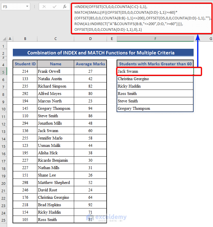
Explanation of the Formula:
C:C is the column from which we want to extract the contents of the list (Student Name in this example).
B:B and D:D are the columns where the criteria lie (Student ID and Average Marks in this example).
B5, C5, and D5 are the cells from where the data starts (just below the Column Headers).
We have multiplied two criteria here: (OFFSET(D5,0,0,COUNTA(D:D)-1,1)>=60)*(OFFSET(B5,0,0,COUNTA(B:B)-1,1)<=200). If you have more than two criteria, multiply accordingly.
Method 3 – Create a Dynamic Drop-Down List Based on Criteria Using the Data Validation ToolSelect any cell in your worksheet and go to Data.
Click on Data Validation under the Data Tools section and select Data Validation.
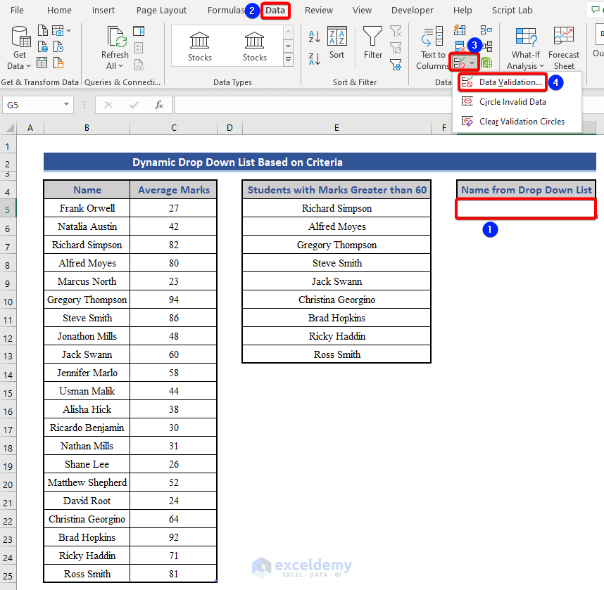
You will get the Data Validation dialogue box.
Under the Allow option, choose List.
Under the Source option, enter the reference of the first cell where the list is in your worksheet along with a HashTag (#)($E$5# in this example).
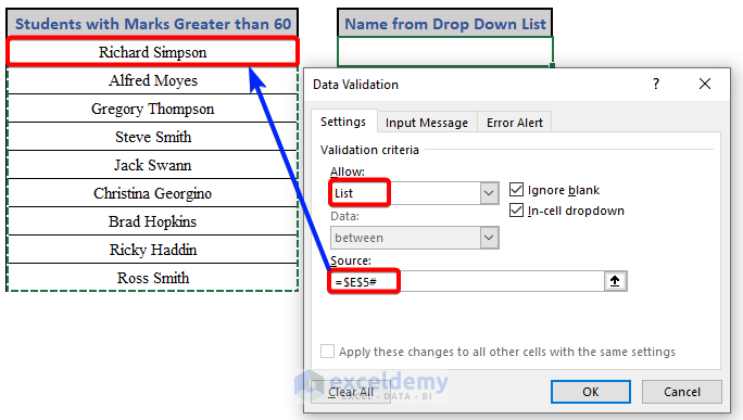
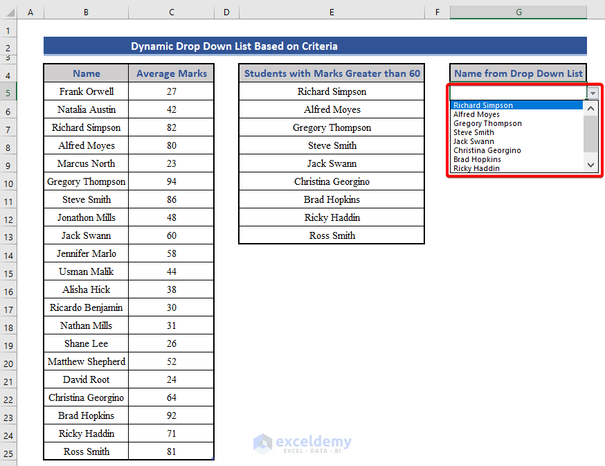
Click OK. You will get a drop-down list in your selected cell.
We modified the dataset and added each student’s favorite games. We’ll list the favorite games of students with marks higher than 60, but will show only the unique results.
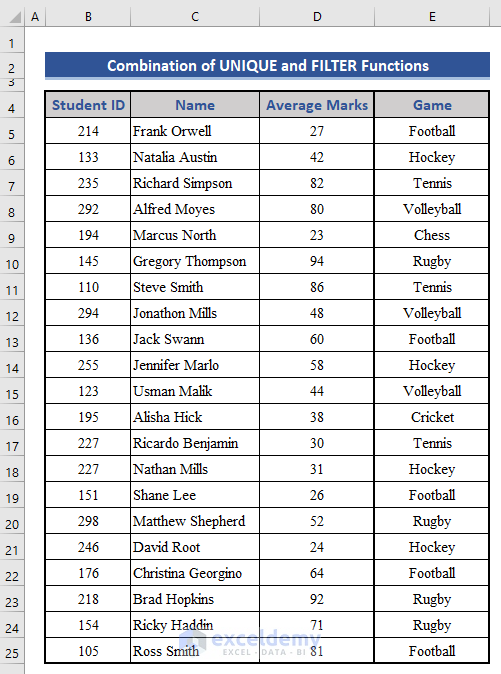
Steps:
Put the following formula in Cell G5.
=UNIQUE(FILTER(E5:E25,(D5:D25>60)))
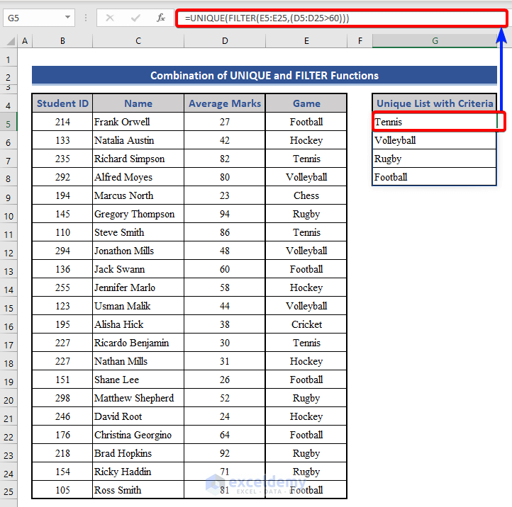
Explanation of the Formula:
FILTER(E5:E25,(D5:D25>60)
This filters the values of Range E5:E25, with a condition that average marks must be above 60.
Result: [Tennis, Volleyball, Rugby, Tennis, Football, Rugby, Rugby, Football]
UNIQUE(FILTER(E5:E25,(D5:D25>60)))
This returns all the unique values from the previous result.
Download the Practice Workbook
Dynamic List Based on Criteria.xlsx
Further Readings<< Go Back to Dynamic List Excel | Excel Drop-Down List | Data Validation in Excel | Learn Excel
SaveSavedRemoved 0
Tags: Dynamic List Excel

Rifat Hassan
Rifat Hassan, BSc, Electrical and Electronic Engineering, Bangladesh University of Engineering and Technology, has worked with the ExcelDemy project for almost 2 years. Within these 2 years, he has written over 250 articles. He has also conducted a few Boot Camp sessions on effective coding, especially Visual Basic for Applications (VBA). Currently, he is working as a Software Developer to develop and deploy additional add-ins to enhance the customers with a more sophisticated experience with Microsoft Office Suits,... Read Full Bio
10 Comments

Roberto
Stops working when there’s two names with the same gradem returns in duplicate instead of showing the two names that have the same grade

Tijs Tijert
I have used your single criteria array formula for older excel versions.
It creates a dynamic list of results I expect with one exeption…
My C:C column contains unique values but the dynamic list is a list where many of the items are duplicated values… why is that?
My criteria column (D:D) does have duplicated values but that shouldn’t be an issue.
What could it be?
{=INDEX(OFFSET(imp_Voorraad!A2;0;0;COUNTIF(imp_Voorraad!A:A)-1;1);MATCH(SMALL(IF(OFFSET(imp_Voorraad!I2;0;0;COUNTIF(imp_Voorraad!I:I)-1;1)>=0;OFFSET(imp_Voorraad!I2;0;0;COUNTIF(imp_Voorraad!I:I)-1;1);””);ROW(A1:INDIRECT(“A”&COUNTIF(imp_Voorraad!I:I;”>=0″))));OFFSET(imp_Voorraad!I2;0;0;COUNTIF(imp_Voorraad!I:I)-1;1);0);1)}

Maruf Islam
Dear Tijs Tijert,
The used formula shouldn’t react this way. Also, I’m not sure what your data and values are that you used as criteria. Kindly email me your dataset to . I’ll try my best to come up with a solution to your problem.
Regards
Maruf Islam
Tijs Tijert
Hi Rifat,
using the single criteria array formula for older excel versions, I get duplicated values in my list, while the source column contains only unique items.
Here is the formula, modified to fit my situation.
{=INDEX(OFFSET(imp_Voorraad!A2;0;0;COUNTIF(imp_Voorraad!A:A)-1;1);MATCH(SMALL(IF(OFFSET(imp_Voorraad!I2;0;0;COUNTIF(imp_Voorraad!I:I)-1;1)>=0;OFFSET(imp_Voorraad!I2;0;0;COUNTIF(imp_Voorraad!I:I)-1;1);””);ROW(A1:INDIRECT(“A”&COUNTIF(imp_Voorraad!I:I;”>=0″))));OFFSET(imp_Voorraad!I2;0;0;COUNTIF(imp_Voorraad!I:I)-1;1);0);1)}
The only difference being that the formula is on another sheet within the workbook, than the source data.
Can you please explain why that is? Because I’ve been staring at this for a while and don’t see it.

martin Maga
Hi all,
I would be great if someone can provide this group with a solution when the values in the criteria columns are repeated (I am trying to use this formula from a list with multiple criterias and both lists have repeated values). The key is that the combination of the two criterias are unique
The other issue I found is that the countifs formula only works if I typed the condition under brakets “”, and the formula doesnt work if I reference to the value to a cell.

Josh
If you use the ‘Unique’ formula around the complete formula, it returns distinct values only.
Eg: =UNIQUE(FILTER(OFFSET(REF!$U$2,0,0,COUNTA(REF!$U:$U)-1,1),(OFFSET(REF!$R$2,0,0,COUNTA(REF!$R:$R)-1,1)=EXAMPLE!$C$7)*(OFFSET(REF!$S$2,0,0,COUNTA(REF!$S:$S)-1,1)=EXAMPLE!$C$8)*(OFFSET(REF!$T$2,0,0,COUNTA(REF!$T:$T)-1,1)=EXAMPLE!$C$9),””))

Md. Shamim Reza
Thanks for your input, Josh. You are absolutely right.
Regards,
Md. Shamim Reza (ExcelDemy Team)

Robbie
How do you write less than 60 but greater than 40 in this formula
=FILTER(OFFSET(C4,0,0,COUNTA(C:C)-1,2),OFFSET(D4,0,0,COUNTA(D:D)-1,1)>=60)
Robbie
How would you do less than 60 but greater than 40 ?
For the first filter offset?
=FILTER(OFFSET(C4,0,0,COUNTA(C:C)-1,2),OFFSET(D4,0,0,COUNTA(D:D)-1,1)>=60)
Thanks
Robbie